library(peRsian)
library(dplyr)
#>
#> Attaching package: 'dplyr'
#> The following objects are masked from 'package:stats':
#>
#>     filter, lag
#> The following objects are masked from 'package:base':
#>
#>     intersect, setdiff, setequal, union
While there is always a qualitative aspect to choosing colors for data visualizations, it’s also possible to quantitatively assess how distinguishable the colors within a palette are.
We can use the colorblindcheck package to evaluate how
distinguishable the colors in each palette are, both under normal vision
and various forms of colorblindness, which is particularly important for
ensuring accessibility in visualizations.
peRsian Palettes
Let’s start by listing all available palettes in the
peRsian package.
names(persian_palettes)
#> [1] "fery" "tehran" "hamburg" "isfahan" "munich" "leyli"
#> [7] "tabriz" "abbas" "reyhaneh" "berlin" "pooran" "hooshang"
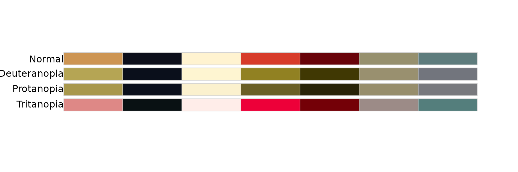
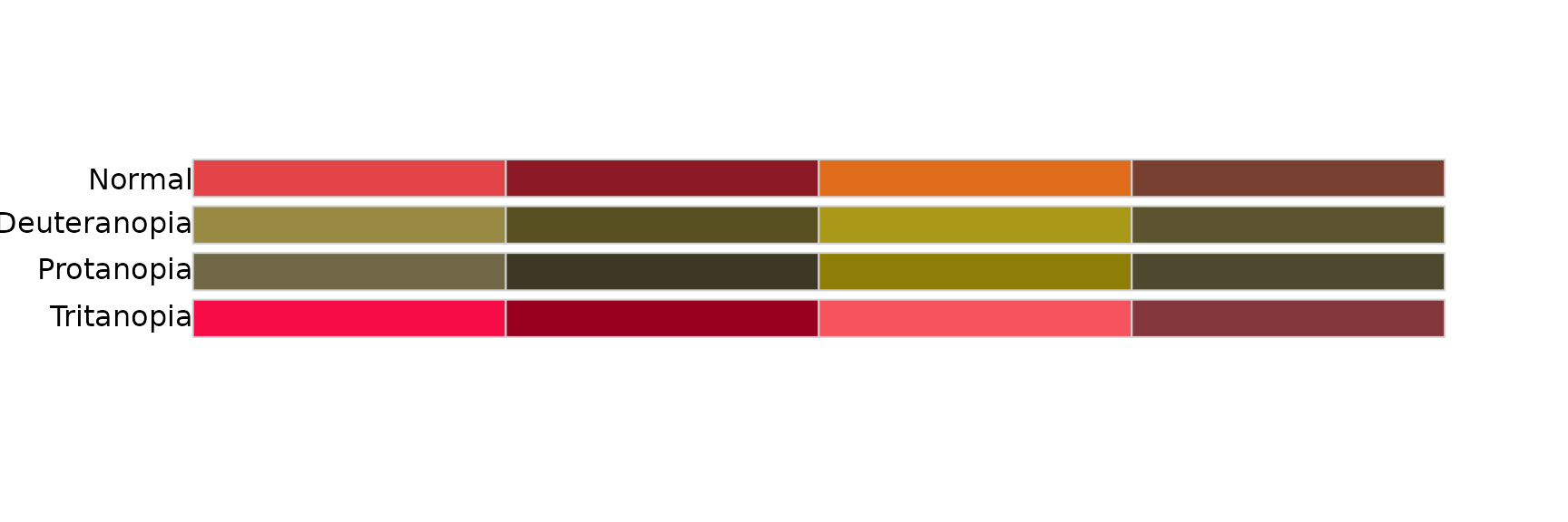
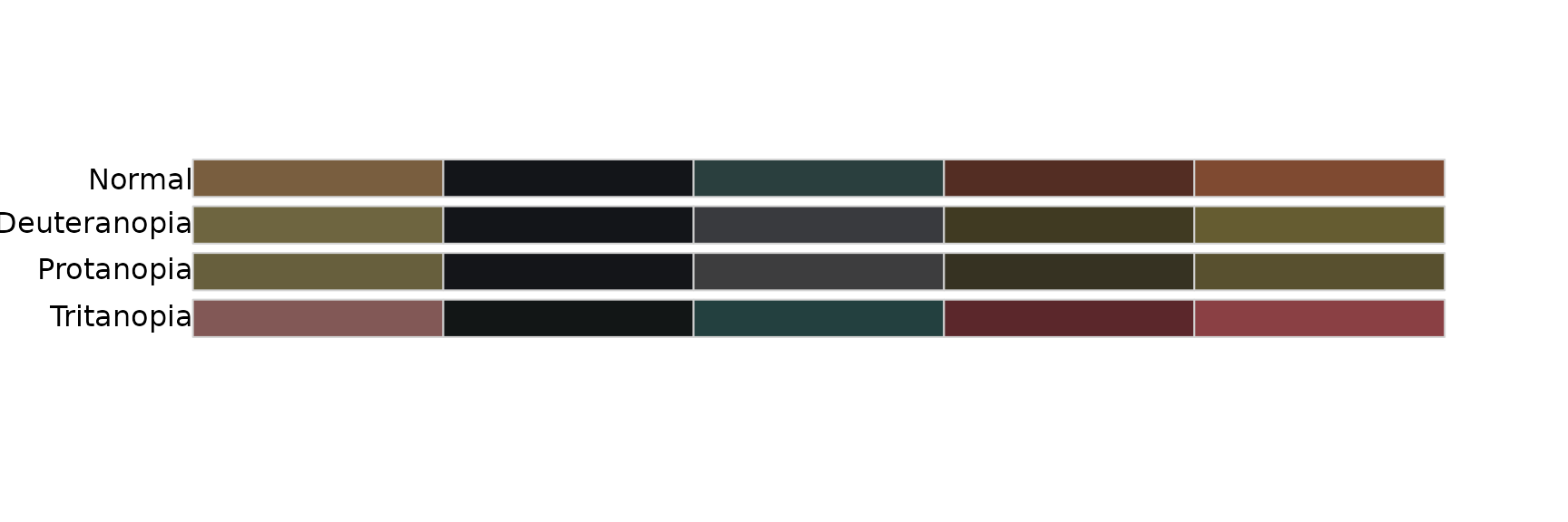
#> [13] "floral"Next, we can have a look at an evaluation of each palette using
colorblindcheck.
# Generate a subjeading and evaluation for each palette
for(palette_name in names(persian_palettes)) {
  cat("\n\n### ", palette_name, "\n\n")

  colors <- persian_palette(palette_name)
  check_results <- colorblindcheck::palette_check(colors, plot = TRUE)

  check_results |>
    knitr::kable(digits = 2) |>
    print()
}
fery
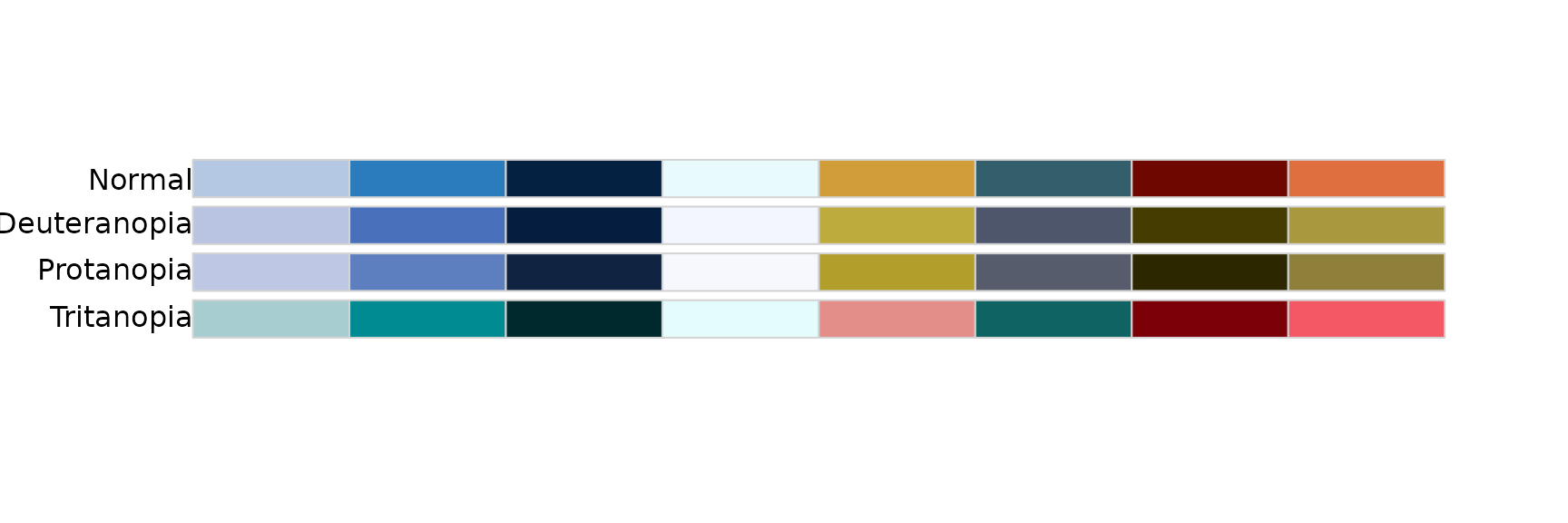
| name | n | tolerance | ncp | ndcp | min_dist | mean_dist | max_dist |
|---|---|---|---|---|---|---|---|
| normal | 8 | 15.32 | 28 | 28 | 15.32 | 44.03 | 81.71 |
| deuteranopia | 8 | 15.32 | 28 | 26 | 6.20 | 43.21 | 82.91 |
| protanopia | 8 | 15.32 | 28 | 26 | 11.93 | 41.82 | 78.92 |
| tritanopia | 8 | 15.32 | 28 | 25 | 11.68 | 44.40 | 77.83 |
tehran
| name | n | tolerance | ncp | ndcp | min_dist | mean_dist | max_dist |
|---|---|---|---|---|---|---|---|
| normal | 8 | 14.66 | 28 | 28 | 14.66 | 37.53 | 71.85 |
| deuteranopia | 8 | 14.66 | 28 | 22 | 2.36 | 28.37 | 60.75 |
| protanopia | 8 | 14.66 | 28 | 21 | 1.59 | 27.80 | 69.35 |
| tritanopia | 8 | 14.66 | 28 | 28 | 15.56 | 38.95 | 71.06 |
hamburg
| name | n | tolerance | ncp | ndcp | min_dist | mean_dist | max_dist |
|---|---|---|---|---|---|---|---|
| normal | 8 | 10.07 | 28 | 28 | 10.07 | 45.91 | 81.62 |
| deuteranopia | 8 | 10.07 | 28 | 25 | 3.48 | 38.97 | 82.43 |
| protanopia | 8 | 10.07 | 28 | 26 | 5.30 | 38.37 | 78.94 |
| tritanopia | 8 | 10.07 | 28 | 27 | 8.17 | 38.28 | 74.83 |
isfahan
| name | n | tolerance | ncp | ndcp | min_dist | mean_dist | max_dist |
|---|---|---|---|---|---|---|---|
| normal | 6 | 17.68 | 15 | 15 | 17.68 | 35.81 | 59.96 |
| deuteranopia | 6 | 17.68 | 15 | 12 | 6.26 | 31.66 | 53.51 |
| protanopia | 6 | 17.68 | 15 | 12 | 8.04 | 31.54 | 54.06 |
| tritanopia | 6 | 17.68 | 15 | 13 | 8.42 | 35.05 | 60.43 |
munich
| name | n | tolerance | ncp | ndcp | min_dist | mean_dist | max_dist |
|---|---|---|---|---|---|---|---|
| normal | 7 | 16.62 | 21 | 21 | 16.62 | 40.90 | 93.83 |
| deuteranopia | 7 | 16.62 | 21 | 18 | 12.14 | 36.13 | 94.46 |
| protanopia | 7 | 16.62 | 21 | 20 | 9.80 | 36.08 | 92.87 |
| tritanopia | 7 | 16.62 | 21 | 21 | 17.31 | 40.04 | 91.23 |
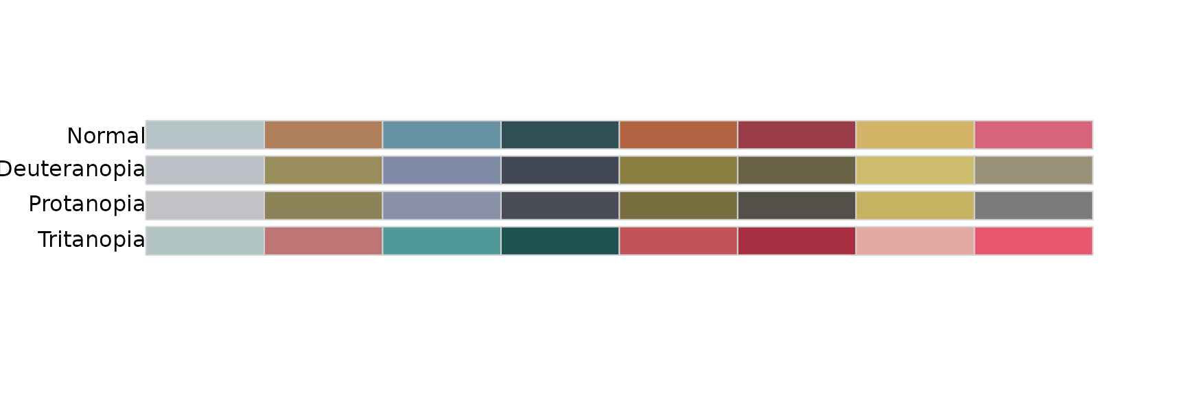
leyli
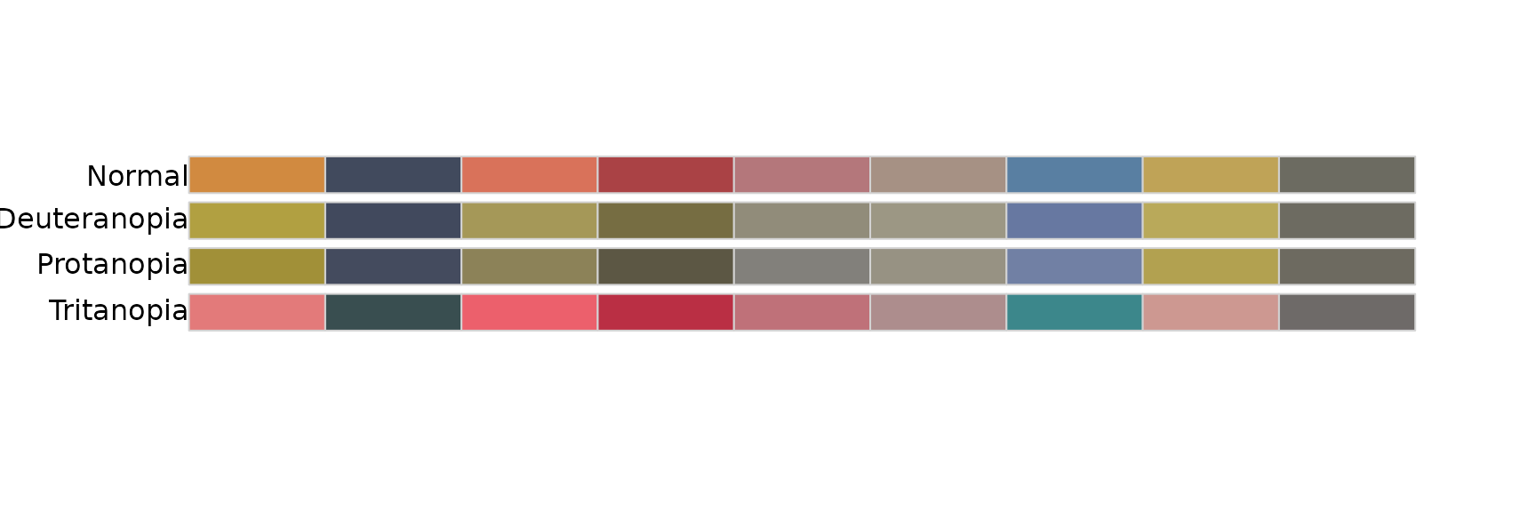
| name | n | tolerance | ncp | ndcp | min_dist | mean_dist | max_dist |
|---|---|---|---|---|---|---|---|
| normal | 9 | 13.12 | 36 | 36 | 13.12 | 28.14 | 49.33 |
| deuteranopia | 9 | 13.12 | 36 | 29 | 3.68 | 23.71 | 51.18 |
| protanopia | 9 | 13.12 | 36 | 29 | 5.58 | 22.47 | 48.22 |
| tritanopia | 9 | 13.12 | 36 | 29 | 5.71 | 26.88 | 55.62 |
tabriz
| name | n | tolerance | ncp | ndcp | min_dist | mean_dist | max_dist |
|---|---|---|---|---|---|---|---|
| normal | 6 | 11.76 | 15 | 15 | 11.76 | 27.51 | 42.58 |
| deuteranopia | 6 | 11.76 | 15 | 14 | 6.20 | 24.18 | 40.79 |
| protanopia | 6 | 11.76 | 15 | 14 | 3.92 | 23.26 | 41.99 |
| tritanopia | 6 | 11.76 | 15 | 14 | 7.73 | 27.65 | 43.73 |
abbas
| name | n | tolerance | ncp | ndcp | min_dist | mean_dist | max_dist |
|---|---|---|---|---|---|---|---|
| normal | 5 | 13.89 | 10 | 10 | 13.89 | 30.28 | 66.85 |
| deuteranopia | 5 | 13.89 | 10 | 9 | 12.26 | 30.30 | 67.68 |
| protanopia | 5 | 13.89 | 10 | 9 | 12.69 | 29.44 | 65.37 |
| tritanopia | 5 | 13.89 | 10 | 10 | 15.66 | 30.42 | 67.36 |
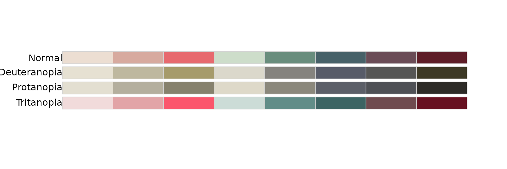
reyhaneh
| name | n | tolerance | ncp | ndcp | min_dist | mean_dist | max_dist |
|---|---|---|---|---|---|---|---|
| normal | 4 | 10.92 | 6 | 6 | 10.92 | 22.66 | 33.38 |
| deuteranopia | 4 | 10.92 | 6 | 4 | 2.83 | 19.44 | 30.52 |
| protanopia | 4 | 10.92 | 6 | 5 | 5.63 | 17.50 | 30.00 |
| tritanopia | 4 | 10.92 | 6 | 4 | 6.85 | 18.31 | 26.09 |
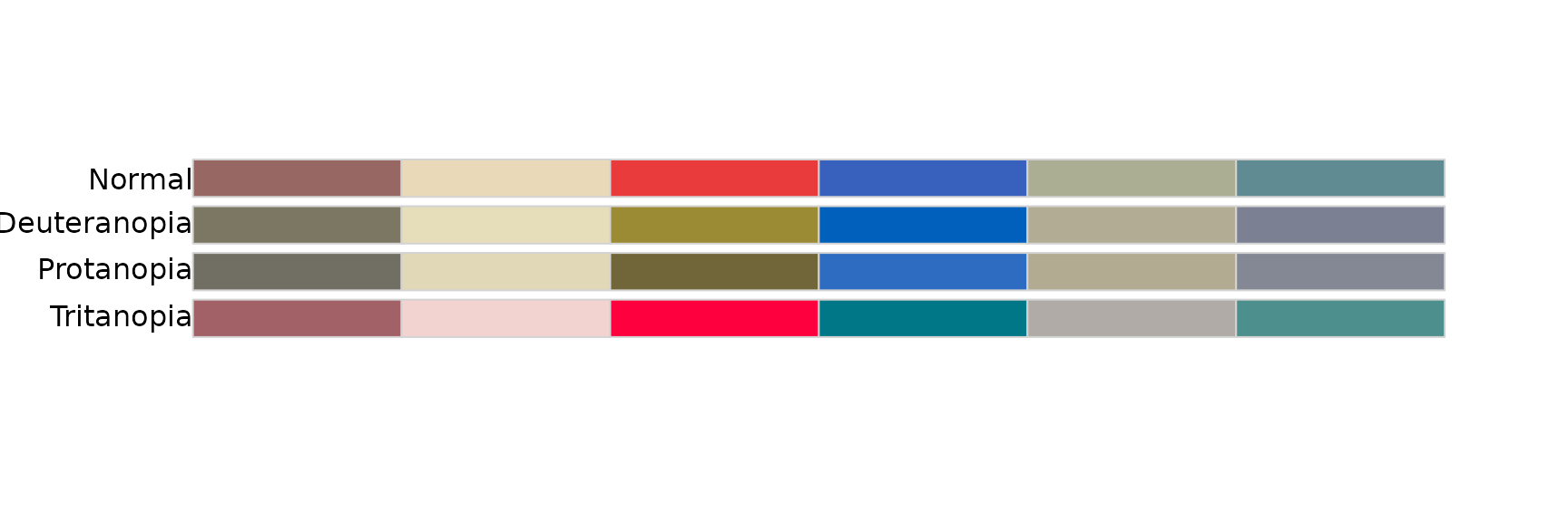
berlin
| name | n | tolerance | ncp | ndcp | min_dist | mean_dist | max_dist |
|---|---|---|---|---|---|---|---|
| normal | 8 | 10.24 | 28 | 28 | 10.24 | 32.75 | 51.84 |
| deuteranopia | 8 | 10.24 | 28 | 26 | 6.27 | 26.29 | 54.16 |
| protanopia | 8 | 10.24 | 28 | 26 | 8.72 | 25.71 | 48.48 |
| tritanopia | 8 | 10.24 | 28 | 25 | 8.07 | 33.11 | 56.35 |
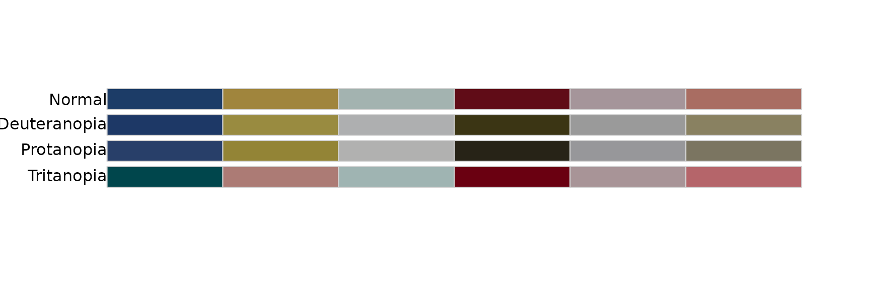
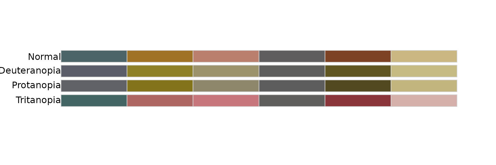
pooran
| name | n | tolerance | ncp | ndcp | min_dist | mean_dist | max_dist |
|---|---|---|---|---|---|---|---|
| normal | 6 | 14.38 | 15 | 15 | 14.38 | 35.29 | 54.31 |
| deuteranopia | 6 | 14.38 | 15 | 14 | 12.71 | 30.26 | 57.05 |
| protanopia | 6 | 14.38 | 15 | 13 | 11.63 | 28.50 | 51.68 |
| tritanopia | 6 | 14.38 | 15 | 14 | 11.93 | 36.11 | 66.67 |
Quantitative Comparison
With the scores produced by colorblindcheck, we can now
perform a proper quantitative analysis to check which palettes meet
certain thresholds and which might need adjustments.
Colorblind-Safety
Let’s compare peRsian with the popular
viridis palette, which has specifically been designed to
handle colorblindness well, to put its the color difference scores into
perspective.
# Helper function to conveniently calculate scores and assign a palette name
calculate_palette_scores <- function(colors, palette_name, ...) {
check_results <- colorblindcheck::palette_check(colors, ...)
cbind(
data.frame(palette = palette_name),
check_results
)
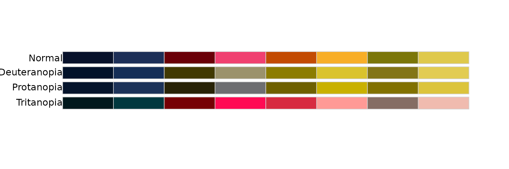
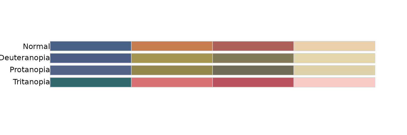
}First, we calculate the scores for viridis.
viridis_scores_df <- calculate_palette_scores(
  viridisLite::viridis(8),
  "viridis",
  plot = TRUE
)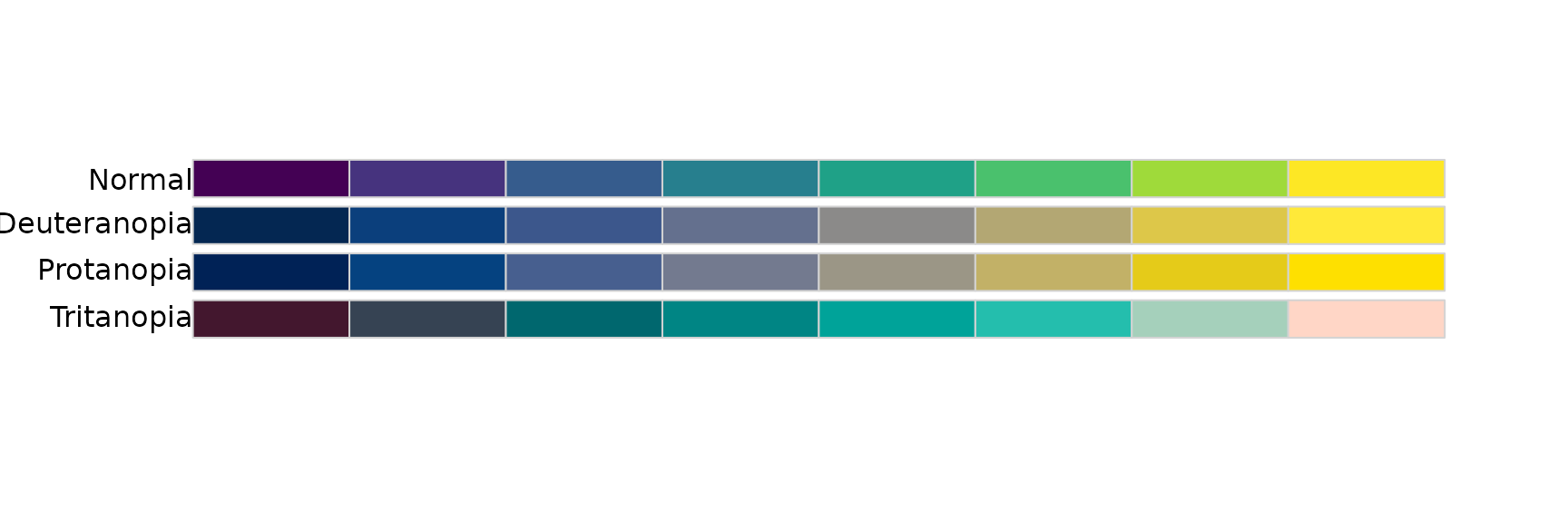
viridis_scores_df |>
knitr::kable(digits = 2)| palette | name | n | tolerance | ncp | ndcp | min_dist | mean_dist | max_dist |
|---|---|---|---|---|---|---|---|---|
| viridis | normal | 8 | 12.45 | 28 | 28 | 12.45 | 46.62 | 100.32 |
| viridis | deuteranopia | 8 | 12.45 | 28 | 24 | 8.43 | 39.97 | 90.16 |
| viridis | protanopia | 8 | 12.45 | 28 | 25 | 5.34 | 41.44 | 93.43 |
| viridis | tritanopia | 8 | 12.45 | 28 | 25 | 8.01 | 38.42 | 76.80 |
Let’s use the smallest difference in viridis as the
threshold to identify which palettes in peRsian we deem
“colorblind-safe”.
viridis_min_score <- min(viridis_scores_df$min_dist)
viridis_min_score
#> [1] 5.339964
# Create a dataframe with scores for all palettes in the package
persian_scores_df <- do.call(rbind, lapply(names(persian_palettes), function(palette_name) {
  calculate_palette_scores(
    persian_palette(palette_name),
    palette_name,
    tolerance = viridis_min_score
  )
}))
Now we can use this information to only mark palettes as colorblind-safe, where the smallest difference is above the threshold across ALL different forms of visual perception.
# Keep only palettes where all entries are above threshold
palettes_above_threshold <- persian_scores_df |>
  group_by(palette) |>
  # Number of comparisons == Number of comparisons above threshold
  filter(all(ncp == ndcp))

colorblind_safe_palettes <- palettes_above_threshold$palette |>
  unique()

colorblind_safe_palettes
#> [1] "fery"     "isfahan"  "munich"   "abbas"    "berlin"   "pooran"   "hooshang"
Let’s also collect the names of all palettes that didn’t make it (use these with caution!).
Ordering Palettes
Finally, we can order all palettes by their minimum color difference (under full vision) to get a better overview of which ones are most distinguishable and which ones may need more work.
persian_scores_df |>
  filter(name == "normal") |>
  arrange(desc(min_dist))
#>     palette   name n tolerance ncp ndcp min_dist mean_dist max_dist
#> 1   isfahan normal 6  5.339964  15   15 17.68255  35.80945 59.96357
#> 2  hooshang normal 4  5.339964   6    6 17.24044  33.19147 48.85390
#> 3    munich normal 7  5.339964  21   21 16.62231  40.89513 93.82743
#> 4      fery normal 8  5.339964  28   28 15.31689  44.03096 81.71196
#> 5    tehran normal 8  5.339964  28   28 14.66018  37.52704 71.85012
#> 6    pooran normal 6  5.339964  15   15 14.38322  35.29478 54.31265
#> 7     abbas normal 5  5.339964  10   10 13.88681  30.27786 66.84959
#> 8     leyli normal 9  5.339964  36   36 13.12127  28.13639 49.32902
#> 9    tabriz normal 6  5.339964  15   15 11.75663  27.51236 42.57928
#> 10 reyhaneh normal 4  5.339964   6    6 10.92315  22.65976 33.38325
#> 11   floral normal 5  5.339964  10   10 10.69823  22.98735 31.90445
#> 12   berlin normal 8  5.339964  28   28 10.24284  32.74987 51.84005
#> 13  hamburg normal 8  5.339964  28   28 10.06714  45.90776 81.61558
Palettes which may need adjustments:
persian_scores_df |>
  filter(name == "normal") |>
  arrange(min_dist)
#>     palette   name n tolerance ncp ndcp min_dist mean_dist max_dist
#> 1   hamburg normal 8  5.339964  28   28 10.06714  45.90776 81.61558
#> 2    berlin normal 8  5.339964  28   28 10.24284  32.74987 51.84005
#> 3    floral normal 5  5.339964  10   10 10.69823  22.98735 31.90445
#> 4  reyhaneh normal 4  5.339964   6    6 10.92315  22.65976 33.38325
#> 5    tabriz normal 6  5.339964  15   15 11.75663  27.51236 42.57928
#> 6     leyli normal 9  5.339964  36   36 13.12127  28.13639 49.32902
#> 7     abbas normal 5  5.339964  10   10 13.88681  30.27786 66.84959
#> 8    pooran normal 6  5.339964  15   15 14.38322  35.29478 54.31265
#> 9    tehran normal 8  5.339964  28   28 14.66018  37.52704 71.85012
#> 10     fery normal 8  5.339964  28   28 15.31689  44.03096 81.71196
#> 11   munich normal 7  5.339964  21   21 16.62231  40.89513 93.82743
#> 12 hooshang normal 4  5.339964   6    6 17.24044  33.19147 48.85390
#> 13  isfahan normal 6  5.339964  15   15 17.68255  35.80945 59.96357